City Learn实战

Glossary

简单介绍一些常用缩写

HVAC (Heating, Ventilation and Air Conditioning): 暖通空调系统。建筑中耗电量最大的部分,也是 CityLearn 中主要的可控负荷。

DHW (Domestic Hot Water): 生活热水。指洗澡、洗手等用途的热水,通常通过电加热器或热泵产生。

PV (Photovoltaic): 光伏(太阳能板)。建筑的分布式电源,产生绿色能源供建筑使用或卖回电网。

EV (Electric Vehicle): 电动汽车。在 CityLearn 中既是负荷,也可以作为移动存储设备。

DER (Distributed Energy Resource): 分布式能源。指部署在用户侧的小型发电或储能设备(如光伏、电池)。

GEB (Grid-interactive Efficient Building): 电网互动高效建筑。指能够根据电网信号动态调整自身用能和储能状态的智能化建筑。

ZNE (Zero Net Energy): 净零能耗。指建筑在一整年内的总能源消耗量与其自身产生的可再生能源量相等的理想状态。

ESS / BESS (Energy / Battery Energy Storage System): 能源存储系统 / 电池储能系统。统指用于储存电能的装置。

TES (Thermal Energy Storage): 蓄热系统。指储存热能或冷能的装置(如水箱、冰蓄冷),通常配合 HVAC 或 DHW 使用。

SoC (State of Charge): 荷电状态。表示电池(或蓄热罐)当前的电量百分比(0%-100%)。

DoD (Depth-of-Discharge): 放电深度。表示电池放出的电量占额定容量的百分比。

RBC (Rule-Based Control): 基于规则的控制。这是最传统的控制方法(如:如果电价便宜就充电),在 CityLearn 中常被用作基准线(Baseline)。

MPC (Model Predictive Control): 模型预测控制。一种基于物理模型的优化算法,需要准确的数学模型来预测未来状态。

RLC (Reinforcement Learning Control): 强化学习控制。CityLearn 的核心研究点,利用智能体(Agent)通过试错学习最优策略。

SAC (Soft-Actor Critic): 一种先进的强化学习算法。在 CityLearn 中非常常用,因为它在连续动作空间下表现稳定且高效。

AI (Artificial Intelligence) & API (Application Programming Interface): AI 是人工智能总称;API 是程序接口,CityLearn 提供了 OpenAI Gym 风格的 API 供你调用环境。

ToU (Time of Use): 分时电价。电费根据时段变化,目的是引导用户在负荷高峰期减少用电。

G2V / V2G (Grid-to-Vehicle / Vehicle-to-Grid): 电网向车辆充电 / 车辆向电网放电。描述电动汽车与电网的双向能量流动。

GHG (Greenhouse Gas): 温室气体。环境指标之一,CityLearn 往往要求在降低成本的同时减少排放。

KPI (Key Performance Indicator): 关键绩效指标。用于衡量你的算法好坏的指标(如:峰值削减率、电费支出、碳排放量等)。

BEPS (Building Energy Performance Simulation): 建筑能效模拟。CityLearn 底层运行的引擎(如 EnergyPlus),用于计算建筑在不同控制下的物理响应。

KPI

实验1 baseline and random baseline(4compared)

直接给出完整代码,主要理清代码的作用

1. 初始化环境

1
2
3
4
5
6
7
8
9
10
11
12
13
14
15
16
17
18
19
20
21
22
23
24
25
26
27
28
# ---init each paras---
# 1. 建筑
BUILDING_COUNT = 2
BUILDINGS = select_buildings(
DATASET_NAME,
BUILDING_COUNT,
RANDOM_SEED,
)
# 2. 激活的观测值
ACTIVE_OBSERVATIONS = ['hour']

# 3. 天数,用于确定开始和结束的时段,平常为了节省时间一般会稍微短一些以加快训练速度
DAY_COUNT = 7
SIMULATION_START_TIME_STEP, SIMULATION_END_TIME_STEP = select_simulation_period(
DATASET_NAME,
DAY_COUNT,
RANDOM_SEED
)

# ---init env---
random_env = CityLearnEnv(
DATASET_NAME, # 数据集名字
central_agent=CENTRAL_AGENT, # True or False,前者为单代理,后者多代理
buildings=BUILDINGS, # 建筑名字,可用于指定
active_observations=ACTIVE_OBSERVATIONS, # 观测值,hour or mins or second
simulation_start_time_step=SIMULATION_START_TIME_STEP, # 从数据集的第n小时开始
simulation_end_time_step=SIMULATION_END_TIME_STEP, # 从数据集的第n小时结束
)

2. 初始化agent

1
2
3
4
# 如果是随机控制,使用RandomAgent,如果是baseline,使用BaselineAgent
random_model = RandomAgent(
random_env
)

3. 重置环境

1
2
3
# reset ur env,和dl中的zero()差不多意思,做就对了,你也不希望第二次训练的时候有第一次训练完的数据吧
# ps,'_'的意思是不需要的返回值
observations, _ = random_env.reset()

4. 训练

1
2
3
4
5
6
while not random_env.terminated:	# 只要模拟没结束,就一直模拟
# 基于当前的observations做出action
actions = random_model.predict(observations)

# 改变量
observations, _, _, _, _ = random_env.step(actions)

介绍一下最后一行,step(actions)为接受到action后,模拟这一个小时内发生的事,与此同时返回五个值

observation:后一个小时的环境

reward:奖励,即奖励函数

terminated:是否结束,是否到达了最后的小时

truncated:是否截断,即因为某些意外原因提前停止

info:其他信息,调试用的额外数据

5. 画图

1
2
3
4
5
# 这是tut的函数,就不赘述了,主要可以看五大KPI判断该策略如何
plot_simulation_summary({
'Baseline': baseline_env,
'Random': random_env,
})

6. 结果

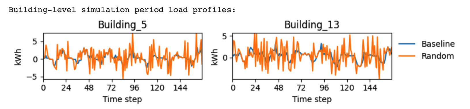
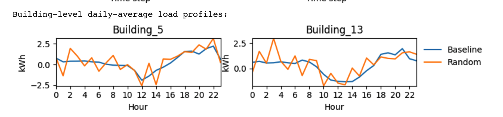
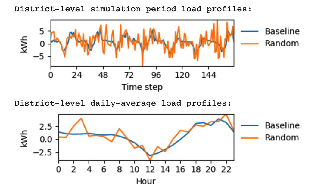
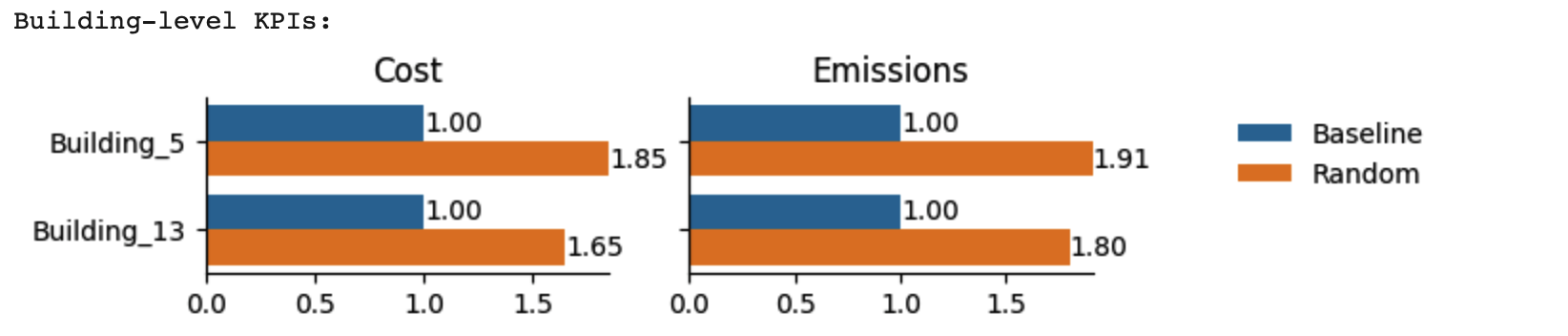
基于画图结果和一部分的KPI,可以得到这些

image-20260106193551601

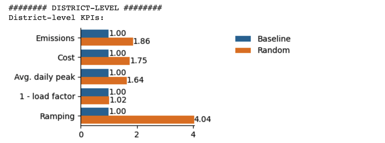
KPI以baseline为准,大于1说明预算超了n%,小于1说明省了n%。这两个都是要求越低越好

image-20260106193614635

image-20260106193645947

Load Profiles越平稳,说明冲放电越平滑,越好。

第一张图为全周期,整个time step的趋势;第二张图为求平均,意思是整个周期内n点点平均效果。可以结合着一起看

image-20260106193703084

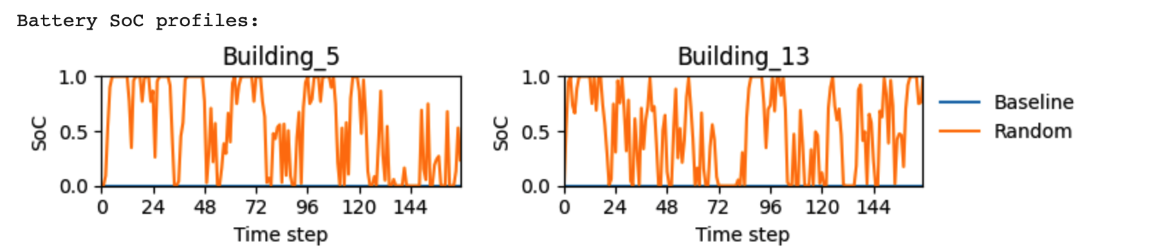
SoC (State of Charge)代表电池的电量百分比[0.0∼1.0].需要有规则的起伏

baseline没有使用到电池因此永远是0,Random看出电池在乱跳,这说明毫无逻辑和效果,同时还会损害电池寿命,对电网造成大冲击

还需要注意,每次充放电都会有能量损失,这也说明浪费了大量的电能。理想情况应该是慢充慢放,前者在电价便宜的时候,后者在贵的时候

image-20260106193728911

给出如下指标

Emissions(碳排放):越低越环保。

Cost(电费成本):越低越省钱。

Avg. daily peak(日均峰值):越低对电网压力越小。

1 - load factor(1 - 负载因子):越低代表用电越均匀高效。

Ramping(爬坡率):越低代表用电量的变化越平缓。

image-20260106193742157

这是sum(所有建筑),和之前的load profiles一个意思,要平滑

实验2 Time-of-Use Rule-Based Control(RoC)

和之前没啥区别,就是多了一个action map,用于控制时间点充放电

1
2
3
4
5
6
7
8
9
10
11
12
13
14
15
16
17
18
19
20
21
22
23
24
25
26
27
28
29
30
31
32
33
34
35
36
37
38
39
40
41
42
43
44
45
46
47
48
49
50
51
# define action map
action_map = {
1: 1/12, # Rule for 1 AM
2: 1/12, # Rule for 2 AM
3: 1/12, # Rule for 3 AM
4: 1/12, # Rule for 4 AM
5: 1/12, # Rule for 5 AM
6: 1/12, # Rule for 6 AM
7: 1/12, # Rule for 7 AM
8: 1/12, # Rule for 8 AM
9: 1/12, # Rule for 9 AM
10: 1/12, # Rule for 10 AM
11: 1/12, # Rule for 11 AM
12: 1/12, # Rule for 12 PM
13: -1/12, # Rule for 1 PM
14: -1/12, # Rule for 2 PM
15: -1/12, # Rule for 3 PM
16: -1/12, # Rule for 4 PM
17: -1/12, # Rule for 5 PM
18: -1/12, # Rule for 6 PM
19: -1/12, # Rule for 7 PM
20: -1/12, # Rule for 8 PM
21: -1/12, # Rule for 9 PM
22: -1/12, # Rule for 10 PM
23: -1/12, # Rule for 11 PM
24: -1/12, # Rule for 12 AM
}

# run inference
rbc_env = CityLearnEnv(
DATASET_NAME,
central_agent=CENTRAL_AGENT,
buildings=BUILDINGS,
active_observations=ACTIVE_OBSERVATIONS,
simulation_start_time_step=SIMULATION_START_TIME_STEP,
simulation_end_time_step=SIMULATION_END_TIME_STEP,
)
rbc_model = HourRBC(rbc_env, action_map=action_map)
observations, _ = rbc_env.reset()

while not rbc_env.terminated:
actions = rbc_model.predict(observations)
observations, _, _, _, _ = rbc_env.step(actions)

# display simulation summary
plot_simulation_summary({
'Baseline': baseline_env,
# Uncomment line below if you have completed Exercise 1
'Random': random_env,
'RBC': rbc_env,
})

其他的几乎一样,就是类名字略有不同

Q- learning

原理

不多说算法原理了,给个p-code

The general Q-Learning algorithm is as follows:

  1. Initialize the Q-table for all state-action pairs.
  2. Set the learning rate $\alpha$ ($0 < \alpha < 1$) and the discount factor $\gamma$ ($0 < \gamma < 1$).
  3. Repeat the following steps for each episode:
    • Observe the initial state $s$.
    • Choose an action $a$ based on the epsilon-greedy policy (a random action is chosen with probability epsilon, $\epsilon$ and the action with the highest Q-value is chosen with probability $1 - \epsilon$).
    • Take the action $a$ and observe the next state $s'$ and the reward $r$.
    • Update the Q-value of the state-action pair $(s,a)$ using the Bellman equation.
    • Set $s = s'$.
  4. Repeat step 3 for a large number of episodes or until convergence is reached.

代码

需要注意的是,citylearn中的内置citylearn.agents.q_learning.TabularQLearning仅支持连续值,该教材遵循base paper,所以将离散值连续化(class:observation_bin_sizes和action_bin_sizes)

1. 初始化环境

1
2
3
4
5
6
7
8
tql_env = CityLearnEnv(
DATASET_NAME,
central_agent=CENTRAL_AGENT,
buildings=BUILDINGS,
active_observations=ACTIVE_OBSERVATIONS,
simulation_start_time_step=SIMULATION_START_TIME_STEP,
simulation_end_time_step=SIMULATION_END_TIME_STEP,
)

2. 离散化

1
2
3
4
5
6
7
8
9
10
11
12
# 定义激活的观测值、动作及其分箱大小
observation_bins = {'hour': 24} # 24个分箱,每个小时都是独立时间
action_bins = {'electrical_storage': 12} # 12个档位,代表充电时间的快慢

# 用来存储每栋建筑对应的分箱规则
observation_bin_sizes = []
action_bin_sizes = []

# 循环,每一栋建筑都离散化
for b in tql_env.buildings:
observation_bin_sizes.append(observation_bins)
action_bin_sizes.append(action_bins)

3. 封装环境

1
2
3
4
5
tql_env = TabularQLearningWrapper(
tql_env,
observation_bin_sizes=observation_bin_sizes,
action_bin_sizes=action_bin_sizes
)

4. 训练Q学习器

1
2
3
4
5
6
7
8
9
10
11
12
13
14
15
16
17
18
19
20
21
22
23
24
25
26
27
28
29
30
31
32
# ----------------- CALCULATE NUMBER OF TRAINING EPISODES -----------------
i = 3 # 一个qtable更新n次
m = tql_env.observation_space[0].n # 24小时
n = tql_env.action_space[0].n # 12个动作
t = tql_env.unwrapped.time_steps - 1
tql_episodes = m*n*i/t
tql_episodes = int(tql_episodes)
print('Q-Table dimension:', (m, n))
print('Number of episodes to train:', tql_episodes)

# ----------------------- SET MODEL HYPERPARAMETERS -----------------------
tql_kwargs = {
'epsilon': 1.0,
'minimum_epsilon': 0.01,
'epsilon_decay': 0.0001,
'learning_rate': 0.005,
'discount_factor': 0.99,
}

# 补丁
tql_env.observation_names = tql_env.unwrapped.observation_names
tql_env.action_names = tql_env.unwrapped.action_names

# ----------------------- INITIALIZE AND TRAIN MODEL ----------------------
tql_model = TabularQLearning(
env=tql_env,
random_seed=RANDOM_SEED,
**tql_kwargs
)

for i in tqdm(range(tql_episodes)):
_ = tql_model.learn()

5. 结果

不怎么好,使用效率等于random策略

SAC

1. 理论

依旧忽略,反正在citylearn里不用Q-table总没错

2. 代码

1. 依旧初始化环境

1
2
3
4
5
6
7
8
sac_env = CityLearnEnv(
DATASET_NAME,
central_agent=CENTRAL_AGENT,
buildings=BUILDINGS,
active_observations=ACTIVE_OBSERVATIONS,
simulation_start_time_step=SIMULATION_START_TIME_STEP,
simulation_end_time_step=SIMULATION_END_TIME_STEP,
)

接着,由于使用了SAC,还需进行以下步骤操作

1
2
3
4
5
6
7
8
# 将环境中的观测值进行归一化操作
sac_env = NormalizedObservationWrapper(sac_env)

# 适配接口,满足stable Baselines3标准
sac_env = StableBaselines3Wrapper(sac_env)

# 初始化 SAC 模型
sac_model = SAC(policy='MlpPolicy', env=sac_env, seed=RANDOM_SEED)

2. 训练SAC模型

1
2
3
4
5
6
7
8
9
10
11
12
13
14
# ----------------- CALCULATE NUMBER OF TRAINING EPISODES -----------------
fraction = 0.25
sac_episodes = int(tql_episodes*fraction)
print('Fraction of Tabular Q-Learning episodes used:', fraction)
print('Number of episodes to train:', sac_episodes)
sac_episode_timesteps = sac_env.unwrapped.time_steps - 1
sac_total_timesteps = sac_episodes*sac_episode_timesteps

# ------------------------------- TRAIN MODEL -----------------------------
for i in tqdm(range(sac_episodes)):
sac_model = sac_model.learn(
total_timesteps=sac_episode_timesteps,
reset_num_timesteps=False,
)

训练出来的结果并不好,因为奖励函数只提供了放电的选项,充电没奖励,所以使用SAC的时候必须还需要自定义奖励函数

3. 奖励函数

主目标是惩罚从电网买电的行为,尤其是电池有电却不放电的情况;同时在电价便宜(21:00 - 08:00)和光伏充足时奖励充电,如下

$$\begin{gathered} r = \sum_{i=0}^n(p_i \times |C_i|) \\ p_i = -(1+sign(C_i) \times SoC_i^{battery}) \end{gathered}$$

由此给出自定义class类

1
2
3
4
5
6
7
8
9
10
11
12
13
14
15
16
17
18
19
20
21
22
23
24
25
26
27
28
29
30
31
32
33
34
35
36
37
38
39
40
41
42
43
44
45
46
47
48
49
50
51
52
53
54
class CustomReward(RewardFunction):
def __init__(self, env_metadata: dict[str, Any]):
r"""Initialize CustomReward.

Parameters
----------
env_metadata: dict[str, Any]:
General static information about the environment.
"""

super().__init__(env_metadata)

def calculate(
self, observations: list[dict[str, int | float]]
) -> list[float]:
r"""Returns reward for most recent action.

The reward is designed to minimize electricity cost.
It is calculated for each building, i and summed to provide the agent
with a reward that is representative of all n buildings.
It encourages net-zero energy use by penalizing grid load satisfaction
when there is energy in the battery as well as penalizing
net export when the battery is not fully charged through the penalty
term. There is neither penalty nor reward when the battery
is fully charged during net export to the grid. Whereas, when the
battery is charged to capacity and there is net import from the
grid the penalty is maximized.

Parameters
----------
observations: list[dict[str, int | float]]
List of all building observations at current
:py:attr:`citylearn.citylearn.CityLearnEnv.time_step`
that are got from calling
:py:meth:`citylearn.building.Building.observations`.

Returns
-------
reward: list[float]
Reward for transition to current timestep.
"""

reward_list = []

for o, m in zip(observations, self.env_metadata['buildings']):
cost = o['net_electricity_consumption']*o['electricity_pricing']
battery_soc = o['electrical_storage_soc']
penalty = -(1.0 + np.sign(cost)*battery_soc)
reward = penalty*abs(cost)
reward_list.append(reward)
reward = [sum(reward_list)]

return reward

再带入到训练中

1
2
3
4
5
6
7
8
9
10
11
12
13
14
15
16
17
18
sacr_env = CityLearnEnv(
DATASET_NAME,
central_agent=CENTRAL_AGENT,
buildings=BUILDINGS,
active_observations=ACTIVE_OBSERVATIONS,
simulation_start_time_step=SIMULATION_START_TIME_STEP,
simulation_end_time_step=SIMULATION_END_TIME_STEP,
reward_function=CustomReward, # assign custom reward function
)
sacr_env = NormalizedObservationWrapper(sacr_env)
sacr_env = StableBaselines3Wrapper(sacr_env)
sacr_model = SAC(policy='MlpPolicy', env=sacr_env, seed=RANDOM_SEED)

for i in tqdm(range(sac_episodes)):
sacr_model = sacr_model.learn(
total_timesteps=sac_episode_timesteps,
reset_num_timesteps=False,
)

站内搜索

没有找到内容!